2. Strange & Complex
2.1 Strange Attractors
Strange attractors rendered with Fractal & Chaotic Flows. Lorenz animations rendered with Gerry's Attraction.
The next logical step is to extend the concepts of iterated systems to multiple-dimensional mappings. Given the results of the previous explorations one can assume that much of the behavior found in the quadratic map will have its analog in higher dimensions and thus we need not introduce an entirely new vocabulary.
Let
ƒ: ℝn → ℝn
be a mapping of ordered n-tuples of real numbers on to themselves. Take the results and feed them back into the map repeatedly. For convenience sake, let's call the n-tuples points and ℝn a space of dimension "n". This procedure generates an orbit of points
p, ƒ(p), ƒ2(p), ƒ3(p), … , ƒn(p), …
in our space from a seed "p". The behavior of orbits in higher dimensions is similar to that in one dimension. Let's look at some of the possibilities in two dimensions.
It's quite easy to devise mappings that illustrate attracting and repelling fixed points. For example,
ƒ: (x, y) → (½x, ½y)
draws all points asymptotically towards the origin while
ƒ: (x, y) → (2x, 2y)
drives them away to infinity. The mapping
ƒ: (x, y) → (−y, +x)
will set every point on its own four-cycle around the origin. Generating a mapping that produces its own unique n-cycle was a bit more difficult. One candidate
ƒ: (x, y) → (cos y−1, sin y−1)
seems to send seeds on to an 11-cycle, but I'm not quite sure. This area of mathematics is highly dependent on computing and I have no computer program for generating arbitrary two-dimensional iterated mappings at my disposal (although I manage it on a programmable calculator).
In higher dimensions, however, attraction and repulsion are not limited to points. An iterative map can collapse on to any structure possible in that dimension. Attractors and repellers can form paths, surfaces, volumes, and their higher dimensional analogs. For example, the two-dimensional map
ƒ: (x, y) → (x, ½y)
attracts all points asymptotically to the x-axis. Likewise, a two-dimensional object can act as a repeller. Such is the case for the map
ƒ: (x, y) → (x2 − y2, 2xy).
Points inside the unit circle head for the origin while those outside fly off to infinity. Points on the circle remain there and thus for this map the unit circle can be considered a fixed repeller.
For comparison, take the set of iterated functions
x → by and y → 1 + x − ay2
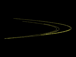
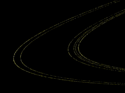
where "a" and "b" are constants set at 1.4 and 0.3 respectively. (Other values are also possible. These just happen to make a good picture.) Those seed values that do not escape to infinity collapse on to the bizarre creature shown below. This is an example of a strange attractor; the Hénon attractor, named after its discoverer, Michel Hénon. Although composed of lines, orbits on this beast do not flow continuously, but hop from one location to another. When drawn, the attractor seems to materialize out of nothing. It is also chaotic. All seed values that converge to the attractor do so in a different manner. Distinct points that are initially separated by even the most minuscule gap will eventually diverge and evolve separately. The Hénon attractor also shows a great deal of fine structure (an infinite amount to be exact). Successive magnifications show an ever increasing degree of detail. Any cross section through an arm of the Hénon attractor is equivalent to a Cantor middle thirds set. What look like lines turn out to be sets of lines on closer inspection. When these lines are magnified they also turn out to be sets of lines. And so on.
 |
 |
 |
 |
Similar bizarre creatures can also be generated using complex numbers. Think back to the time when you first learned about square roots. Most likely you were told that one cannot find the square root of a negative number. Even though your calculator will probably agree with this statement, it's not really true. It's not that the answer can't be found, but that it can't be expressed in terms of the so-called real numbers of day to day existence. To get around this problem, a new class of numbers were postulated. These were then unfortunately named the imaginary numbers. I say unfortunately named because the term imaginary implies that these numbers do not really exist or that they are somehow inferior to the real numbers. I think it would have been better to call them the "extraordinary numbers" to distinguish them from the "ordinary numbers" we associate with ordinary types of calculations. After all, how often does the typical human need to find the square root of negative one?
Unfortunate names aside, adding the imaginary numbers to mathematics makes the subject all that more interesting. A number that is partially real and partially imaginary is said to be complex. Complex numbers can be represented as the sum of the two parts or as a coordinate pair where "i" squared is equal to negative one.
z = x + iy = (x, y)
Thus, a complex iterated mapping
ƒ(z) → z
is equivalent to a two dimensional mapping
ƒ(x,y) → (x,y)
that just happens to follow the rules of complex arithmetic. Start with a complex function or just take any old real function and seed it with a complex number, grind the results through the function over and over again, and plot the resulting orbit on the real-imaginary plane.
When this process is applied to the function
| ƒ: (z) → a + bz exp | ⎡ ⎢ ⎣ |
i | k − p | ⎤ ⎥ ⎦ |
| 1 + |z|2 |
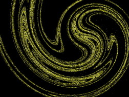
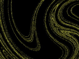
a strange attractor emerges — the Ikeda attractor. With a suitable choice of parameters all sorts of different swirled and folded patterns can be made. The example shown below is reminiscent of the turbulences found in rising trails of smoke (a = 0.85, b = 0.9, k = 0.4, p = 7.7). Like the Hénon attractor, the Ikeda attractor shows a fine structure that just never quits. That's what makes these objects "strange".
 |
 |
 |
 |
Although they might look like just pretty pictures, all of the strange attractors on this page have their origin in the study of real or idealized physical systems. Hénon's attractor arose from the study of perturbations in asteroid orbits and Ikeda's from a nonlinear optical system. The systems studied by Hénon and Ikeda were two dimensional, but there is no reason why physical systems or the strange attractors that may arise from them should be limited to two dimensions.
The most famous strange attractor is undoubtedly the Lorenz attractor — a three dimensional object whose body plan resembles a butterfly or a mask. The Lorenz attractor, named for its discoverer Edward N. Lorenz, arose from a mathematical model of the atmosphere.
Imagine a rectangular slice of air heated from below and cooled from above by edges kept at constant temperatures. This is our atmosphere in its simplest description. The bottom is heated by the earth and the top is cooled by the void of outer space. Within this slice, warm air rises and cool air sinks. In the model as in the atmosphere, convection cells develop, transferring heat from bottom to top.
The state of the atmosphere in this model can be completely described by three time-evolving variables
| x = | the convective flow |
| y = | the horizontal temperature distribution |
| z = | the vertical temperature distribution |
with three parameters describing the character of the model itself
| σ [sigma] = | the ratio of viscosity to thermal conductivity |
| ρ [rho] = | the temperature difference between the top and bottom of the slice |
| β [beta] = | the width to height ratio of the slice |
and three ordinary differential equations describing the appropriate laws of fluid dynamics
| dx/dt = | σ(y − x) |
| dy/dt = | ρx − y − xz |
| dz/dt = | xy − βz |
Although greatly simplified, we have here a model that is still impossible to solve analytically and tedious to solve numerically. One that would require an army of graduate students scribbling on hundreds of pages of paper working around the clock. It probably wouldn't have been solved in 1960 if it weren't for the fact that Lorenz had something better than an army of human computers — the improbably named Royal McBee — an early electronic computer whose vacuum tubes could perform sixty multiplications a second, round the clock, without taking a break or asking for time off. The Royal McBee made it possible to do numerical calculations that would have been cruel and unusual punishment to the human calculators. One could configure it in the morning and let it run for hours or days, printing out solutions for later analysis. This is how Lorenz discovered chaos.
In the course of doing this I wanted to examine some of the solutions in more detail. I had a small computer in my office then so I typed in some of the intermediate conditions which the computer had printed out as new initial conditions to start another computation and then went out for awhile. When I came back I found that the solution was not the same as the one I had before. The computer was behaving differently. I suspected computer trouble at first. But I soon found that the reason was that the numbers I had typed in were not the same as the original ones. These were rounded off numbers. And the small difference between something retained to six decimal places and rounded off to three had amplified in the course of two months of simulated weather until the difference was as big as the signal itself. And to me this implied that if the real atmosphere behaved in this method then we simply couldn't make forecasts two months ahead. The small errors in observation would amplify until they became large (Lorenz interviewed by Peitgen).
In order to conserve paper, the computer was instructed to round the solutions before printing them. Thus, a solution like 0.506127 was printed as 0.506. Even in 1960 computers gave answers with more significant digits than were required for most problems. An error of one part in four thousand should hardly have been significant. Tolerances aren't anywhere near this tight in construction or manufacturing or life in general. If you built your home using a meter stick that was 999.7 millimeters long would your house collapse? Would it be askew? Would you ever notice anything was wrong with it?
When it comes to the weather, the answer to that last question was "yes." After enough time had elapsed, the tiny error introduced by dropping the digits after the thousandths place became an error as large as the range of possible solutions to the system. Lorenz called this the Butterfly Effect, or rather it became known as the Butterfly Effect as the result of an accident in publishing.
Well this really came from a paper that I gave called "Can the flap of a butterfly's wings in Brazil stir up a tornado in Texas?" (Actually the title was one that someone had given to me. I probably would have picked a seagull instead of a butterfly. It works the same way.) I pointed out at the beginning of the talk that this wasn't really supposed to be a facetious question. And that if it were true then certainly if a butterfly's wings could stir up a tornado, then a butterfly could be equally effective in preventing a tornado that otherwise would have happened…. So the real question was can very small influences lead in due time to very big changes? But it's apparently because of the title of this paper that it's become known as the butterfly effect. (Lorenz interviewed by Peitgen)
A butterfly was chosen as its effect on atmospheric dynamics must surely be small and a tornado was chosen as its meteorological size is about as extreme as one can get. Extremely small perturbations in a system may result in an outcome as large as the difference between a tornado occurring or not occurring. What is informally known as the Butterfly Effect is more properly known as sensitive dependence on initial conditions (usually shortened to sensitive dependence). It is an essential characteristic of a chaotic system. Sensitive dependence is chaos.
| Initial value used as seed | Truncated, intermediate value used as seed | ||
| time | temperature | time | temperature |
|---|---|---|---|
| 01 | 10.338268 | 01 | - |
| 02 | −5.380525 | 02 | - |
| 03 | 10.017644 | 03 | - |
| 04 | −5.322683 | 04 | - |
| 05 | −14.052872 | 05 | - |
| 06 | 2.757209 | 06 | - |
| 07 | −7.552990 | 07 | - |
| 08 | 6.621076 | 08 | - |
| 09 | −8.084304 | 09 | - |
| 10 | [omitted] | 10 | - |
| 11 | −9.952578 | 11 | −9.952000 |
| 12 | −5.981163 | 12 | −6.120309 |
| 13 | −13.023813 | 13 | −12.646284 |
| 14 | 0.041168 | 14 | −0.724073 |
| 15 | 9.314363 | 15 | 11.848833 |
| 16 | 4.558919 | 16 | −1.204758 |
| 17 | 7.375924 | 17 | 6.826824 |
| 18 | −14.856846 | 18 | 13.773982 |
| 19 | −0.246566 | 19 | 1.474239 |
Actually, the system of equations Lorenz used can also exhibit other types of behavior that are not chaotic. Given the right combination of parameters, some orbits will settle down after enough iterations to a fixed value — finite or infinite. You don't hear about these solutions as most everyone would agree that they couldn't possibly represent any real weather system. The only interesting solutions of the Lorenz system are the ergodic ones — those that visit every point in some region, or more accurately, those that will eventually approach arbitrarily close to every point within that region. Real weather changes. It never settles down and it also never repeats. Sure there are days that are alike, but they are never exactly alike. The Lorenz model is a success in that it there are outcomes that are similar, but they never repeat themselves.
Real weather is also bounded; that is, there are limits to the kinds of weather one would expect as long as the earth, sun, and atmosphere were never to experience any changes in character. The tropics can get hot, but they'll never get hot enough to melt lead. Storm winds may be stiff, but they'll never exceed the speed of sound. If the Lorenz model is accurate it should exhibit these kinds of behavior. The problem is, how can we determine if this is the case? The answer is not to look at the raw numbers, but to look at a plot of the values that emerge. If a picture is worth a thousand words then a movie should at least be worth a couple hundred words.
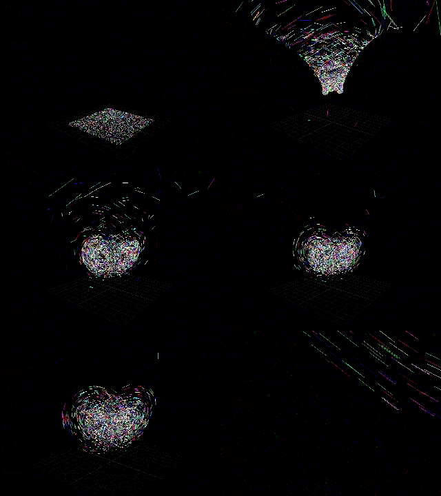 |
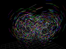
In the movie above, 5000 weather states with different two dimensional temperature profiles and no initial convection eventually evolve into sequences that are somewhat similar. The snapshots below capture this activity from several different angles.
 |
 |
 |
 |
 |
 |
 |
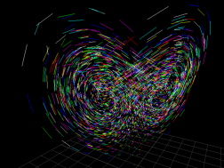 |
The Lorenz attractor is indeed bounded. Interestingly enough, the shape to which all orbits converge looks something like the proverbial butterfly of the paper Lorenz presented in Texas. Although it also looks something like a mask as the image below illustrates.
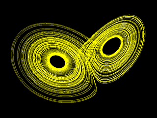 |
While the attractor appears as two warped disks, their actual structure is far more complex. Recall how the numbers Lorenz generated with the Royal McBee were ergodic (approaching every possible value) and aperiodic (never repeating). In much the same manner that what appear to be lines in the Hénon attractor turn out to be pairs of lines, what appear to be disks in the Lorenz attractor turn out to be layers of disks. The Lorenz attractor is less like two CDs melted together and more like two puff pastries baked together. A geometric figure of this sort with an infinite level of detail is called a fractal. (This is an informal definition for now. A more formal one will arise in a later chapter.) Fractals are the second essential characteristic of chaos. Sensitive dependence, you will recall, is the first. Chaos always results in the formation of a fractal, but not all fractals are associated with chaos. Probably, the right way to say it is that chaos makes fractals.
A puff pastry, by the way, is made by starting with a ball of dough, rolling it out flat, folding it over like a newspaper, rolling that out flat again, folding the result, and so on. The mathematical equivalent of rolling and folding and rolling and folding is the origin of sensitive dependence in the Lorenz attractor as well as in the much simpler quadratic mapping (which we will revisit in the remaining sections of this chapter). Imagine a spot of food coloring added to a sheet of pastry dough. After a few repetitions of folding and rolling it's easy to see how that initially small spot would wind up stretched so thin that it occupied a much larger area and then folded so many times that it occupied nearly every layer. Two pieces of colored dough that were initially near to each other could, after the appropriate number of repetitions, have any separation between them allowed by the dimensions of the dough. Or in Lorenz' appropriately technical language "until the difference was as big as the signal itself." When translated into weather-speak this became the butterfly effect — the flapping of a butterfly's wings in South America can make the difference between a tornado forming or not forming in Texas some time later.
Unfortunately, the ability to determine whether or not such a thing would come to pass is impossible to say. All measurements will be uncertain at some level (whether it is at the third digit or the thirty billionth digit is of little importance) and all errors will amplify to the point where they render long range prediction useless. All of them!


