4. Measuring Chaos

4.4 Lyapunov Space
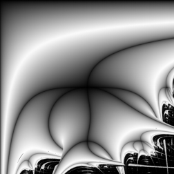
Lyapunov diagrams rendered with Lyapunov.
We have seen how the logistic equation can exhibit behavior reminiscent of a simple harmonic oscillator (equilibrium states, parameter dependent periodicity, Lyapunov stability) and a damped harmonic oscillator (asymptotic stability; over, under, and critical damping). What analog, if any, is there of the driven harmonic oscillator in discrete dynamics? The logistic equation is much richer than the harmonic oscillator in that it can also exhibit chaotic behavior. An exploration of the driven logistic equation should likewise prove interesting.
The differential equation for the damped harmonic oscillator was driven by the addition of a time-dependent force. In a similar manner, a time-dependent population modifier could be tacked on to the left side of the logistic equation. What this would correspond to in our model is uncertain. Individuals would be entering and leaving our population with some kind of regularity. This implies the existence of some source external to the local population. Such behavior is the case with some pack animals. When a pack has too many members some of them (usually the servile males) leave to join other groups. This is one method of driving the logistic equation, but not the one to be discussed in this chapter. I am curious whether anyone has ever explored this possibility.
A second way of looking at the driven and damped components of the harmonic oscillator is as a modification of the system's energy. Driving an oscillator by applying a time-dependent force and damping it by applying a velocity-dependent force does work on the system and changes its energy dynamically. The dissipative term always reduces the system's energy while the driving term can either increase or decrease it. In the logistic equation
ƒ(x) = rx (1 − x)
we will mimic this by driving the growth parameter "r" in a time-dependent manner.
Interestingly enough, this method of driving a dynamic system by varying its parameter was first studied in continuous systems. Take the example of a swing. How can one force it to oscillate? The traditional method is by leaning backward or forward in the seat at the extreme points on the arc. This is equivalent to applying a time-dependent force to the swing and is of limited usefulness at large amplitudes. The second method is to stand in the seat and oscillate up and down by squatting. This is equivalent to driving the oscillator by varying its most important parameter; the effective length. This method alone will not get the swing started, but any small deviation from the equilibrium position will be quickly amplified. I once saw this demonstrated by a college professor in a large lecture hall. He was able to increase the amplitude to the point where he was nearly parallel to the ground at the extreme ends of the cycle. This placed him about twelve to fifteen feet above the floor within about a half dozen swings.
Since the growth parameter always seeks to increase the population it differs from the driving force of the oscillator. However, the (1 − x) term acts as a damping factor to restrain the rate of change of the population. It differs from the damping factor "gamma" of the harmonic oscillator in that its power to slow growth is absolute. As long as the growth factor is within the limits of realistic behavior, the population may not exceed the carrying capacity of the environment.
How do we now go about driving the time-dependent parameter of a difference equation; one in which time per se is never a factor? Just as with the driven harmonic oscillator, the time-dependent component of the driven logistic equation will mimic the solution of the simple logistic equation. In a discrete dynamical system, periodicity exists as a set of "n" discrete sequenced values that the system will cycle through repeatedly:
{x1, x2, … , xn, x1, x2, … , xn, …}.
The driven logistic equation in difference form will thus be written as
An+1 = rn mod pAn(1 − An)
where r0, r1, … ,rp−1 are the parameters and "p" is the period.
We are now ready to study the behavior of the driven logistic equation. We will do this by examining the Lyapunov exponent of the system as a function of the parameter sequence. For simplicity sake we shall limit ourselves to only two distinct parameter values; call them "a" and "b". Thus
{ab}, {aab}, {abaabab} = {(aba)2b}
are all acceptable sequences {rn} while {abc} is not. This restriction enables us to plot this information graphically. If we let "a" and "b" be the axis in some parameter space (call it the Lyapunov space) we can then calculate the exponent for all allowable combinations of parameters (those in the interval (0, 4)). The Lyapunov exponent λ(a, b) now behaves as a scalar field like temperature or altitude and can be displayed in much the same manner. To each value we will assign a specific color. The color scheme used will be the one devised by Mario Markus in his 1990 Computers in Physics article. Assign white to all points where lambda equals zero and black to all points where lambda is greater than zero. This highlights the transition from order to chaos. For points where lambda is less than zero assign a shade of gray such that values close to zero are nearly white while those close to λ = −∞ are nearly black. Assign black again to any point where λ = −∞ (i.e., the superstable points and cycles).
A collection of Lyapunov diagrams is presented below. Note that as the number of terms in the sequence increases, so too does the number of superstable arms meeting at a point. Note also that asymmetric sequences produce asymmetric diagrams. Harder to notice, but intuitively obvious is that each diagram has the same cross section through the diagonal line a = b. When this happens, the situation reduces to the bifurcation diagram.
 |
 |
 |
 |
 |
 |
 |
 |
The diagram below is a zoom in Lyapunov space for the sequence {ab}. The first snapshot corresponds to the window with (0, 0) in the upper left hand corner and (4, 4) in the lower right. The black regions below and to the right are chaotic while the largest black stripe is the family of superstable points. The center of the "x" is the point (2, 2). Other stripes correspond to families of superstable n-cycles. The flotsam in the chaotic regime corresponds to stable islands of odd-multiple periodicity. Again, note the self-referential nature of the islands to the whole picture. The blob in the last picture has the same swallow-tail configuration as the entire space as well as its own atoll of stable islets.
 |
The most impressive feature of these diagrams is their three-dimensional appearance. The swallow-tail structure in the last picture, when rendered in more detail, looks like a solid blob and the superstable arms appear to cross over one other. When the sequence is reversed to {ba} the crossing of the arms reverses. At these locations, we have the coexistence of two attractors, each of which may have a different period. Markus found extremely high levels of basin interleaving in more complicated sequences. The ultimate fate of an orbit (that is, to which basin it will attract) depends on which parameter value we start with. There is no analog of this behavior in the driven harmonic oscillator (although this does not preclude such behavior from being found in other continuous systems). We have uncovered a new type of phenomena.
In some cases of overlap, one arm is accompanied by what looks like a shadow. Again, by reversing the sequence, or starting the sequence with the second term instead of the first the direction of overlap will reverse. This is more extreme than just choosing between one basin and another as it includes points that will switch from order (white or gray) to chaos (black). Markus found that by randomly switching between two paired sequences (e.g., between {ab} and {ba} or {abaabb} and {baabba}) orbits in these regions would head for the superstable attractor rather than the chaotic regime. Graphically, the shadows would disappear and the diagram would take on a fuzzy, hybridized appearance. This is the phenomenon of noise-induced order. Chaos with randomness yields stability. Truth is stranger than fiction.